4.12. pyopus.optimizer.psade — Box constrained parallel SADE global optimizer

Box constrained parallel SADE global optimizer (PyOPUS subsystem name: PSADEOPT)

SADE stands for Simulated Annealing with Differential Evolution.

A provably convergent (parallel) global optimization algorithm.

The algorithm was published in [psade].

psade

Olenšek J., Tuma T., Puhan J., Bűrmen Á.: A new asynchronous parallel global optimization meth od based on simulated annealing and differential evolution. Applied Soft Computing Journal, vol. 11, pp. 1481-1489, 2011.

class pyopus.optimizer.psade.ParallelSADE(function, xlo, xhi, debug=0, fstop=None, maxiter=None, populationSize=20, pLocal=0.01, Tmin=1e-10, Rmin=1e-10, Rmax=1.0, wmin=0.5, wmax=1.5, pxmin=0.1, pxmax=0.9, seed=0, minSlaves=1, maxSlaves=None, spawnerLevel=1)

Parallel SADE global optimizer class

If debug is above 0, debugging messages are printed.

The lower and upper bound (xlo and xhi) must both be finite.

populationSize is the number of inidividuals (points) in the population.

pLocal is the probability of performing a local step.

Tmin is the minimal temperature of the annealers.

Rmin and Rmax are the lower and upper bound on the range parameter of the annealers.

wmin, wmax, pxmin, and pxmax are the lower and upper bounds for the differential evolution’s weight and crossover probability parameters.

seed is the random number generator seed. Setting it to None uses the builtin default seed.

All operations are performed on normalized points ([0,1] interval corresponding to the range defined by the bounds).

If spawnerLevel is not greater than 1, evaluations are distributed across available computing nodes (that is unless task distribution takes place at a higher level).

See the BoxConstrainedOptimizer for more information.

accept(xt, ft, ip, itR)

Decides if a normalized point xt should be accepted. ft is the corresponding cost function value. ip is the index of the best point in the population. itR is the index of the point (annealer) whose temperature is used in the Metropolis criterion.

Returns a tuple (accepted, bestReplaced) where accepted is True if the point should be accpeted and bestReplaced is True if accepting xt will replace the best point in the population.

check()

Checks the optimization algorithm’s settings and raises an exception if something is wrong.

contest(ip)

Performs a contest between two random points in the population for better values of the temperature and range parameter. The first point’s index is ip. The second point is chosen randomly.

generateTrial(xip, xi1, delta1, delta2, R, w, px)

Generates a normalized trial point for the global search step.

A mutated normalized point is generated as

xi1 + delta1*w*random1 + delta2*w*random2

where random1 and random2 are two random numbers from the [0,1] interval.

A component-wise crossover of the mutated point and xip is performed with the crossover probability px. Then every component of the resulting point is changed by a random value generated from the Cauchy probalility distribution with parameter R.

Finally the bounds are enforced by selecting a random value between xip and the violated bound for every component of the generated point that violates a bound.

Returns a normalized point.

generateTrialPrerequisites()

Generates all the prerequisites for the generation of a trial point.

Choosed 5 random normalized points (xi1..xi5) from the population.

Returns a tuple comprising the normalized point xi1, and two differential vectors xi2-xi3, xi4-xi5.

initialPopulation(Np)

Constructs and returns the initial population with Np members.

initialTempRange()

Chooses the values of the range and temperature parameters for the annealers.

classmethod localStep(xa, fa, d, origin, scale, rnum1, rnum2, evf, args)

Performs a local step starting at normalized point xa with the corresponding cost function value fa in direction d. Runs remotely.

The local step is performed with the help of a quadratic model. Two or three additional points are evaluated.

The return value is a tuple of three tuples. The furst tuple lists the evaluated normalized point, the second one lists the corresponding cost function values and the third one the corresponding annotations. All three tuples must have the same size.

Returns None if something goes wrong (like a failure to move a point within bounds).

reset(x0=None)

Puts the optimizer in its initial state.

If it is a 2-dimensional array or list the first index is the initial population member index while the second index is the component index. The initial population must lie within bounds xlo and xhi and have populationSize members.

If the initial point x0 is a 1-dimensional array or list, Np-1 population members are generated. Point x0 is the Np-th member. See the initialPopulation() method.

If x0 is None the Np members of the initial population are generated automatically.

run()

Run the algorithm.

selectControlParameters()

Selects the point (annealer) whose range, temperature, differential operator weight and crossover probability will be used in the global step.

Returns the index of the point.

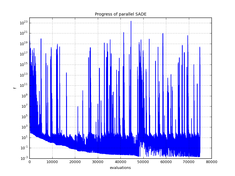
Example file psade.py in folder demo/optimizer/

Read Using MPI with PyOPUS if you want to run the example in parallel.

# Optimize SchwefelA function with PSADE
# Collect cost function and plot progress
# Run the example with mpirun/mpiexec to use parallel processing

from pyopus.optimizer.psade import ParallelSADE
from pyopus.problems import glbc
from pyopus.optimizer.base import Reporter, CostCollector, RandomDelay
from numpy import array, zeros, arange
from numpy.random import seed
from pyopus.parallel.cooperative import cOS
from pyopus.parallel.mpi import MPI
# Import after MPI is imported so that only the master process fires up the GUI thread
from pyopus.plotter import interface as pyopl

if __name__=='__main__':
	cOS.setVM(MPI())
	
	ndim=30
	
	prob=glbc.SchwefelA(n=ndim)
	slowProb=RandomDelay(prob, [0.001, 0.010])
	
	opt=ParallelSADE(
		slowProb, prob.xl, prob.xh, debug=0, maxiter=75000, seed=None
	)
	cc=CostCollector()
	opt.installPlugin(cc)
	opt.installPlugin(Reporter(onIterStep=1000))
	opt.reset()
	opt.run()
	cc.finalize()
	
	f1=pyopl.figure()
	pyopl.lock(True)
	if pyopl.alive(f1):
		ax=f1.add_subplot(1,1,1)
		ax.semilogy(arange(len(cc.fval)), cc.fval)
		ax.set_xlabel('evaluations')
		ax.set_ylabel('f')
		ax.set_title('Progress of parallel SADE')
		ax.grid()
		pyopl.draw(f1)
	pyopl.lock(False)
	
	print("x=%s f=%e" % (str(opt.x), opt.f))
	
	pyopl.join()
	
	cOS.finalize()