The cost function
In this example we will try to find the global minimum of a cost function defined by an analytical expression. So this is strictly mathematical case, which will demonstrate the power of the optimize command. The cost function has to have more local minima. Therefore it is a hard task for any optimisation method. Appropriate two dimensional cost function is defined by equation below.

To make optimisation problem even more complicated we will add an implicit constraint, defined by equation:

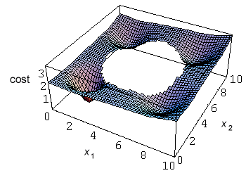
Because our analytic cost function is only two dimensional, it can be plotted. From the figure below it is obvious that if the initial guess is not chosen well the optimisation method can be easily trapped in one of the local minima.

The optimisation process
In
SPICE OPUS the optimisation parameters
x1 and
x2 can be two dc voltages of an independent voltage sources. The cost function can be calculated by a non-linear dependent voltage source. Here is the "netlist" for our mathematical circuit (part of the
analytical_case.cir file):
*** Analytical Case ***

.control
optimize parameter 0 @v1[dc] low 0 high 10 initial 10
optimize parameter 1 @v2[dc] low 0 high 10 initial 10
optimize implicit 0 ((v(1) - 5)^2 + (v(2) - 5)^2) gt 9
optimize analysis 0 op
optimize cost v(out)
optimize method complex
.endc

v1 1 0 dc 10V
v2 2 0 dc 10V

b1 out 0 v = 2.5 + ((v(1) - 2)^2 + (v(2) - 2)^2) / 100
  + - 2 * exp(- ((v(1) - 2)^2 + (v(2) - 2)^2))
  + - exp(- ((v(1) - 2)^2 + (v(2) - 8)^2) / 2)
  + - exp(- ((v(1) - 8)^2 + (v(2) - 2)^2) / 2)
  + - exp(- ((v(1) - 8)^2 + (v(2) - 8)^2) / 2)

.end
Notice that the global minimum is near point
x1 = 2,
x2 = 2 and the initial guess for the optimisation process is picked very inconvenient at point
x1 = 10,
x2 = 10. Therefore most of the optimisation methods do not find the global minimum and get trapped in one of the local minima. The constrained simplex method is one of the few which overcomes this problem.
Spice Opus 1 -> source analytical_case.cir
Circuit: *** Analytical Case ***
Spice Opus 2 -> optimize
Time needed for optimisation: 0.660 seconds
Number of iterations: 111
Lowest cost function value: 5.001213e-001
Optimal values:
v1	dc	=	2.006811e+000
v2	dc	=	2.003741e+000
Spice Opus 3 -> _
More than two dimensions
We also try to find the global minimum of a similar four dimensional cost function as the one optimised above. The cost function has 15 local minima at all corners of a four dimensional cube and the global minimum near point x1 = x2 = x3 = x4 = 2 (see file analytical_case.cir for details). Again a four dimensional sphere was placed in the centre of the cube as an implicit constraint. The global minimum was found by the constrained simplex optimisation method in 296 iterations.
Five dimensional case
Let us now consider next five dimensional case. The cost function is defined by

where r is the distance from the centre of the cube

and the implicit constraint is defined by

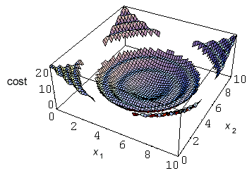
We can plot the two dimensional version of this cost function.

In this case the optimising methods can be trapped in one of the channels. The global minimum at point x1 = x2 = x3 = x4 = x5 = 5 was found in 452 iterations.
The initial_guess option
If we do not find the global minimum in our first optimisation run we can obtain further information about the cost function by new optimisation runs in a part of the parameter space where the cost function was not checked yet. To do this we have to choose an initial point away from all known points from the previous optimisation runs. This can be done automatically by the
initial_guess option. The option is set by
optimize options command.
optimize options initial_guess 10
When we set the initial_guess option the starting point for the next optimisation run will be determined according to all known points.
Let us now return to our four dimensional case above. Now we will use the steepest descent optimisation method instead of constrained simplex. The steepest descent method has local character and therefore gets trapped in local minima. The initial_guess option will be used. We just perform some optimisation runs and the results are different minima of the cost function. The global minimum is found in the second optimisation run.