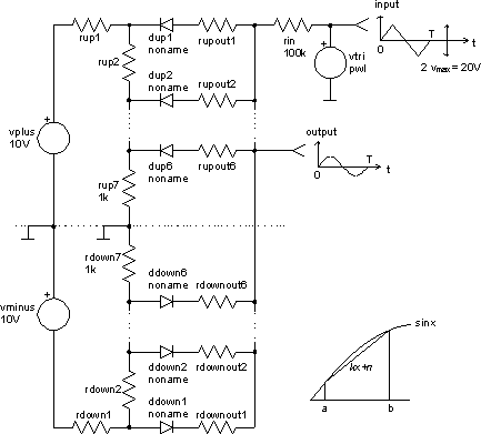
Let us now consider a circuit depicted below, which converts triangular signal waveform to sine waveform. We would like to set the resistances in the circuit so that the purest possible sine signal can be obtained at the output.

We will try to solve circuit analytically and calculate the values of the unknown resistors. The first problem is where to choose the break points. The relative error on one section is:

assuming b - a < p/2.

This result tells us that the best choice are equidistant break points. If we assume ideal diodes with cutin voltage ~ 0.5V and r_upi << r_upoutj, than resistor values can be calculated (see teble below).

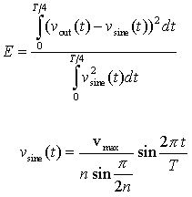
Now we will optimise our circuit with the optimize command. Because of symmetry of the circuit we will observe only one half of the circuit in one quarter of a period. In this case we have 12 parameters to optimise r_up1 ... r_up6, r_upout1 ... r_upout6. The explicit constraints (see table below) are set around analytically calculated values. There are no implicit constraints. Let the cost function be defined as normalised square area between the real and ideal response:

It is a positive scalar and the circuit with ideal sine response would have its value zero.

The initial point of optimisation method is approximately the center of the explicitly constrained parameter space.

Table 1: Resistor values (all values are rounded)

	analytic	explicit constraint	initial	optimised
rupout1	17.0kW	10 ÷ 20 kW	15kW	10.1kW
rupout2	87.6kW	50 ÷ 150 kW	100kW	98.5kW
rupout3	216kW	100 ÷ 300 kW	200kW	244kW
rupout4	432kW	200 ÷ 600 kW	400kW	500kW
rupout5	828kW	400 ÷ 1200 kW	800kW	1.07MW
rupout6	1.89MW	1 ÷ 3 MW	2MW	2.62MW
rup1	4.57kW	2.5 ÷ 7.5 kW	5kW	4.50kW
rup2	511W	250 ÷ 750 W	500W	578W
rup3	824W	400 ÷ 1200 W	800W	883W
rup4	1.09kW	500 ÷ 1500 W	1kW	1.13kW
rup5	1.31kW	500 ÷ 1500 W	1kW	1.18kW
rup6	1.46kW	500 ÷ 1500 W	1kW	1.22kW

We ran the optimisation with different optimisation methods from the same initial point. The parameters of all methods were set to their default values. So results (see table below) with the particular method could be improved by fine tuning method parameters. Anyway we can see that gradient methods have local character. They are quickly trapped in a local minimum, which can be just a consequence of numerical noise. Random and genetic algorithm search across whole parameter space but they need a lot of iterations to get satisfying results. Direct search methods performed better. Hooke-Jeeves's method was the best among direct search methods for this example. On the other hand Powell's method converged very fast and constrained simplex method gave slightly better result, but it did not manage to converge in 4000 iterations. Time needed for optimisation was measured on 200Mhz Pentium personal computer running Windows 95. Optimal parameter values obtained by Hooke-Jeeves's method are shown in the table above.

Table 2: Optimisation statistics

	number of iterations	cost value	time [s]
initial point		4.05 10-3
analitical point		3.26 10-5
steepest descent	174	1.72 10-5	4.07
newton	480	2.28 10-3	10.6
davidon_fletcher_powell	103	9.44 10-5	2.30
monte_carlo	4000	1.07 10-5	88.2
grid_search	4097	3.98 10-3	85.9
axis_search	871	8.47 10-6	19.6
powell	362	8.81 10-6	8.07
hooke_jeeves	1625	3.39 10-6	35.3
complex	4001	3.21 10-6	89.5
genetic	2550	1.03 10-5	60.6

To check if we improved analytically calculated circuit, we will take a closer look after the harmonic distortion of the output signal. We can see (table below) that optimisation method starting from initial circuit, which is worse than analytical circuit, gave better results than analytically calculated. The reason is in taking real diodes into account instead of ideal diodes in analytic circuit.

Table 3: Harmonic distortion (normalised magnitudes)

	initial	analytic	optimised
f0	1	1	1
3f0	1.91 10-2	4.59 10-3	9.23 10-4
5f0	2.01 10-3	2.87 10-3	5.44 10-4
7f0	4.29 10-4	1.16 10-3	4.04 10-4
9f0	1.17 10-3	1.27 10-3	1.19 10-3