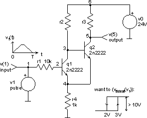
In this example a simple schmitt trigger circuit will be optimised by optimize command. We are looking for the values of the two resistors r2 and r3 in the circuit shown below. We want to have switching voltages at 3V (up) and at 2V (down). The high and low level output voltages must differ for at least 10V.

Here is the netlist of the circuit (part of schmitt_trigger.cir file):

*** schmitt trigger ***

v0 6 0 dc 24V
v1 1 0 dc 0 pulse 0 5V 0 5s 5s 1s

r1 1 2 10k
r2 3 6 12k
r3 5 6 8k
r4 4 0 1k

q1 3 2 4 2n2222
q2 5 3 4 2n2222

.model 2n2222 npn (is=19f bf=150 vaf=100 ikf=.18 ise=50p ne=2.5
  + br=7.5 var=6.4 ikr=12m isc=8.7p nc=1.2 rb=50 re=.4 rc=.3
  + cje=26p tf=.5n cjc=11p tr=7n xtb=1.5 kf=0.032f af=1)

.end

First we have to define some explicit as well as one implicit constraint. The explicit constraints are obvious since we know that the resistor values can't possibly lie outside the intervals:

And because we want a difference between high and low voltage at least 10V, the implicit constraint is:

The most important part of any optimisation is certainly the cost function. In our case we want the cost function to reflect the accuracy of switching voltages. Since we intend to do transient analyses, we define the cost function as a normalised square area between the real and ideal response:

The cost function must be a positive scalar and will be minimised during the optimisation procedure. The ideal value is zero, in which case the switching voltages are exactly at 3V and 2V. Transient response v₅ has to be transformed because of the numerical noise in it. So instead of v₅ we will use the expression below, where boolean operator > is used.

Using normalised ideal response v_5ideal-norm the cost function can be further simplified.

Because we are interested only in vector v(5), we will not save all other vectors calculated in a particular analysis. save command defines which vectors will be saved. Then the circuit's netlist is loaded by source command. We will also define a vector ideal in a const plot, which is never destroyed. This vector is in fact v_5ideal-norm and will be needed for calculating the cost function.

Spice Opus 1 -> source (filename with netlist of the circuit)
Circuit: *** schmitt trigger ***
Spice Opus 2 -> save v(5)
Spice Opus 3 -> let ideal = (vector(11001) gt 2999) and
  (vector(11001) lt 9001)

First we have to define the parameters, which can vary in the optimisation process. Those are resistance of element r2 and resistance of element r3. This can be done by optimize parameter command. At the same time we will give the explicit constraints for both parameters and the initial point (r2 = 12kW, r3 = 8kW), where the optimisation algorithm will start.

Spice Opus 4 -> optimize parameter 0 element @r2[resistance]
  low 10k high 30k initial 12k
Spice Opus 5 -> optimize parameter 1 element @r3[resistance]
  low 1k high 50k initial 8k

We also have to define the commands, which will be executed in every iteration. Those commands have to provide data for computing the value of the cost function and for verifying the implicit constraints (in this example there is one implicit constraint). To compute the cost function the transient response is needed, which has to be linearised. So we will define tran and linearize commands by optimize analysis command.

Spice Opus 6 -> optimize analysis 0 tran 1ms 11s
Spice Opus 7 -> optimize analysis 1 linearize 1ms

The expressions for all implicit constraints (in our case only one) and cost function have to be defined next. We will use the optimize implicit and optimize cost commands. The expressions have to be written in standard Nutmeg language. So we have to convert the equations above into Nutmeg expressions.

Spice Opus 8 -> optimize implicit 0 v(5)[5500] - v(5)[0] gt 10
Spice Opus 9 -> optimize cost
  mean(abs((v(5) gt ((v(5)[5500] + v(5)[0]) / 2)) - ideal))

The optimisation method and its parameters can be defined by optimize method command. We will choose the Hooke and Jeeves's method (hooke_jeeves). The method has two parameters: alpha defines the step magnifying factor, and epsilon defines the stop criteria, when the optimisation algorithm stops. We will leave both parameters at their default values 1.3 and 0.1. The algorithm therefore stops when the size of the last step is less than 0.1% of parameter space in each direction.

Spice Opus 10 -> optimize method hooke_jeeves

Now we are ready to start the optimisation algorithm by optimize command without parameters. When the algorithm converges the results and some statistics are written.

Spice Opus 11 -> optimize
Time needed for optimisation: 255.300 seconds
Number of iterations: 83
Lowest cost function value: 9.090083e-005
Optimal values:
@r2[resistance]	=	1.801962e+004
@r3[resistance]	=	2.000019e+004

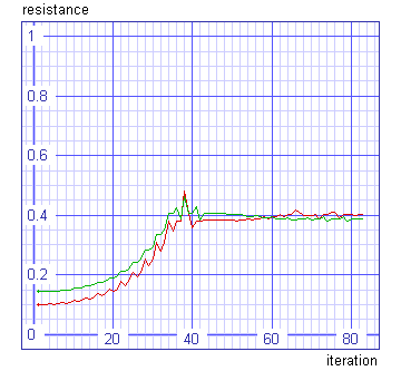
It is interesting to see how did the parameter values (both resistances) travel around the parameter space during the optimisation. The normalised values of the resistances can be plotted by plot command.

Spice Opus 12 -> plot (r2_resistance-1e4)/2e4 (r3_resistance-1e3)/49e3
  ylimit 0 1 xlabel iteration ylabel resistance

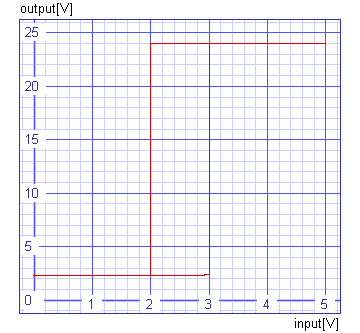
Lets verify the switching voltages. We have to plot output versus input voltage.

Spice Opus 13 -> save v(1)
Spice Opus 14 -> tran 1ms 11s
Spice Opus 15 -> delete 2
Spice Opus 16 -> plot v(5) vs v(1) ylimit 0 25 xlabel input[V]
  ylabel output[V]

We can see that the switch up and switch down voltages are exactly at 3V and 2V.

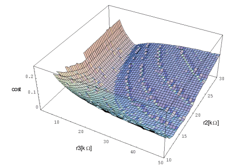
In our case parameter space is two dimensional, so the cost function could be plotted. First the cost function has to be calculated over the entire explicitly constrained parameter space. We can do this with parameter_space "method". Let us calculate 50 times 50 points in the parameter space.

Spice Opus 17 -> optimize method parameter_space npts0 50 npts1 50
Spice Opus 18 -> optimize
Time needed for optimisation: 7519.470 seconds
Number of iterations: 2500
Lowest cost function value: 1.727116e-003
Optimal values:
r2      resistance      =       1.816327e+004
r3      resistance      =       2.000000e+004
Spice Opus 19 -> _

The result of this optimisation is text file with values of the cost function. This file can be read into Mathematica and cost function over explicitly constrained parameter space can be plotted there.

Implicit constraint is violated in the area where the cost function is not plotted. The channels are consequence of numerical errors, which take place because the time step in transient analysis is too long. It is determined automatically. We could define its maximum length, but one analysis would take more time then.

The input file (schmitt_trigger.cir) comes with the installation. It does not do exactly the same steps which are described above.