In this example a simple transistor amplifier is optimised by optimize command. The amplifier is built around standard bipolar npn transistor 2n3510 in orientation with common emitter. The circuit is shown in figure below.

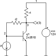
Here is the netlist of the circuit (part of amplifier.cir file):

*** Simple amplifier ***

vcc 1 0 dc 12V
i1 2 0 dc 0A

r1 1 3 45k
r2 2 3 195k

q1 3 2 0 2n3510

.model 2n3510 npn
  + bf=100 br=1.35e-4 xtb=1.5 is=8.35e-14 eg=1.11 cjc=9.63e-12
  + cje=9.47e-12 rb=16.7 rc=1.66 vaf=90 tf=1e-10 tr=1.27e-4
  + cjs=1e-15 vjs=0.8 mjs=0.5 var=100 ise=4.77e-11 isc=1e-16
  + ikf=0.18 ikr=1000 irb=1 rbm=0 vtf=1000

.end

We want to amplify input current. Its amplitude does not exceed 100uA:

The amplifier is supplied with direct voltage vcc = 12V. The resistors r1 and r2 determine the operating point and the feedback factor of the amplifier. They also have an influence on all other properties of the amplifier (input and output impedance, gain, degree of non-linearity, upper frequency limit, noise spectrum etc.). The output voltage is in general given by equation:

We are interested in non-linear distortion of the output. We can estimate, that all other properties will be in acceptable boundaries, if the resistances r1 and r2 are inside these intervals:

Relations above defines explicit constraints. These constraints are often defined by technology. So, in this example, we search for the couple r1 and r2 inside these intervals, which give the most linear response and a gain factor defined as:

must satisfy the implicit constraint:

at the same time. The amplification and non-linear distortion will be studied on direct transfer function, which is also competent for low frequencies. Circuit analyses in all four corners of parameter space will be performed for illustration and are depicted below. We will change resistor values with alter command and will do four dc analyses. Because we are interested only in vector v(3), we will not save all other vectors calculated in a particular analysis. save command defines which vectors will be saved.

Spice Opus 1 -> source (filename with netlist of the circuit)
Circuit: *** Simple amplifier ***
Spice Opus 2 -> save v(3)
Spice Opus 3 -> alter r1 resistance = 5k
Spice Opus 4 -> alter r2 resistance = 20k
Spice Opus 5 -> dc i1 -100uA 100uA 10uA
Spice Opus 6 -> alter r1 resistance = 50k
Spice Opus 7 -> dc i1 -100uA 100uA 10uA
Spice Opus 8 -> alter r2 resistance = 200k
Spice Opus 9 -> dc i1 -100uA 100uA 10uA
Spice Opus 10 -> alter r1 resistance = 5k
Spice Opus 11 -> dc i1 -100uA 100uA 10uA
Spice Opus 12 -> plot dc1.v(3) dc2.v(3) dc3.v(3) dc4.v(3) xlabel i1[A]
  ylabel v(3)[V] title 'Direct Transfer Functions'

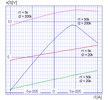
We can see that the r1 = 50k and r2 = 200k corner is far from linear and therefor probably not optimal. A unique criterion, which values of r1 and r2 are the best, is needed in the first place. In our case the rate of non-linearity have to be defined.

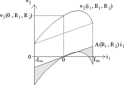
A line through the origin of the co-ordinate system with slope A(r1, r2) is drawn. Then square difference from centred transfer function v3(i1, r1, r2) - v3(0, r1, r2) is calculated. Square difference is integrated over entire interval and normalised with integral of squared ideal response.

So our cost function is defined as:

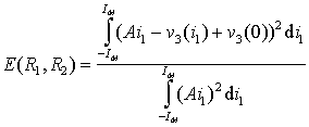
Last expression gives a formula for numerical computing of cost function.

First we have to define the parameters, which can vary in the optimisation process. Those are resistance of element r1 and resistance of element r2. This can be done by optimize parameter command. At the same time we will give the explicit constraints for both parameters and the initial point (r1 = 45k, r2 = 195k), where the optimisation algorithm will start.

Spice Opus 13 -> optimize parameter 0 @r1[resistance]
  low 5k high 50k initial 45k
Spice Opus 14 -> optimize parameter 1 @r2[resistance]
  low 20k high 200k initial 195k

We also have to define the commands, which will be executed in every iteration. Those commands have to provide data for computing the value of the cost function and for verifying the implicit constraints. In our example a dc analysis provides all data needed. So we define only one dc command by optimize analysis command.

Spice Opus 15 -> optimize analysis 0 dc i1 -100uA 100uA 10uA

The expressions for all implicit constraints (in our case only one) and cost function have to be defined next. We will use the optimize implicit and optimize cost commands. The expressions have to be written in standard Nutmeg language. So we have to convert the equations above into Nutmeg expressions.

Spice Opus 16 -> optimize implicit 0
  (v(3)[20] - v(3)[0]) / (2 * 100uA) gt 20k
Spice Opus 17 -> optimize cost (3 * mean((((v(3)[20] - v(3)[0]) /
  (2 * 100uA)) * sweep - v(3) + v(3)[10])^2)) /
  (((v(3)[20] - v(3)[0]) / (2 * 100uA))^2 * (100uA)^2)

Optimisation methods should find the minimum of a cost function with respect to explicit and implicit constraints. The constrained simplex optimisation method will be used in this example. It is one of the most robust direct optimisation methods and is fairly simple. The optimisation method and its parameters can be defined by optimize method command. We will choose the constrained simplex method (complex) and leave all method's parameters at their default values.

Spice Opus 18 -> optimize method complex

Now we are ready to start the optimisation algorithm by optimize command without parameters. When the algorithm converges the results and some statistics are written.

Spice Opus 19 -> optimize
Complex: stopped, simplex small enough
Time needed for optimisation: 0.300 seconds
Number of iterations: 62
Lowest cost function value: 8.738595e-004
Optimal values:
@r1[resistance]	=	2.041547e+004
@r2[resistance]	=	3.529963e+004

Is optimised amplifier really linear? We can verify that. We will do one more dc analysis and plot the result to see the linearity of the response.

Spice Opus 20 -> dc i1 -100uA 100uA 10uA
Spice Opus 21 -> plot v(3) xlabel i1[A] ylabel v(3)[V]
  title 'Response of Optimal Circuit'

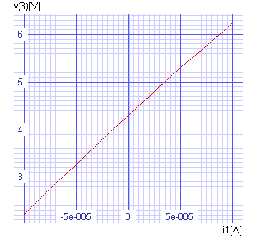
In our case parameter space is two dimensional, so the cost function could be plotted. First the cost function has to be calculated over the entire explicitly constrained parameter space. We can do this with parameter_space "method". Let us calculate 50 times 50 points in the parameter space.

Spice Opus 22 -> optimize method parameter_space npts0 50 npts1 50
Spice Opus 23 -> optimize
Time needed for optimisation: 35.260 seconds
Number of iterations: 2500
Lowest cost function value: 8.886914e-004
Optimal values:
@r1[resistance]	=	2.244898e+004
@r2[resistance]	=	3.469388e+004
Spice Opus 24 -> _

The result of this optimisation is text file with values of the cost function. This file can be read into Mathematica and cost function over explicitly constrained parameter space can be plotted there.

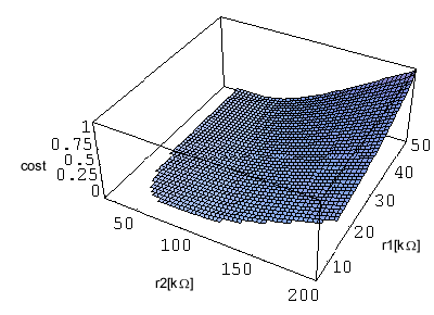
Implicit constraint is violated in the area where the cost function is not plotted.

The input file (amplifier.cir) comes with the installation. It does not do exactly the same steps which are described above.