11.7.2. Running the task and viewing the results

We can start the task by choosing Task/Start locally or Task/Start on cluster from the main menu. It is recommended that this task is startedin parallel mode as it can take quite a while to complete. We can view the log and the results database while the run is in progress.

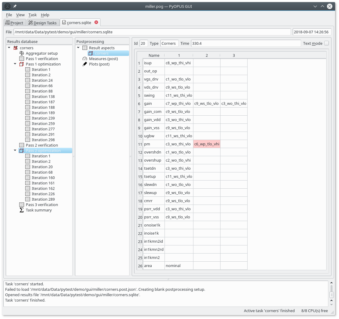
The corners used in the second optimization pass. We can see that only one corner has been added to those used in the first pass (c6_wp_tlo_vhi for the pm performance measure).

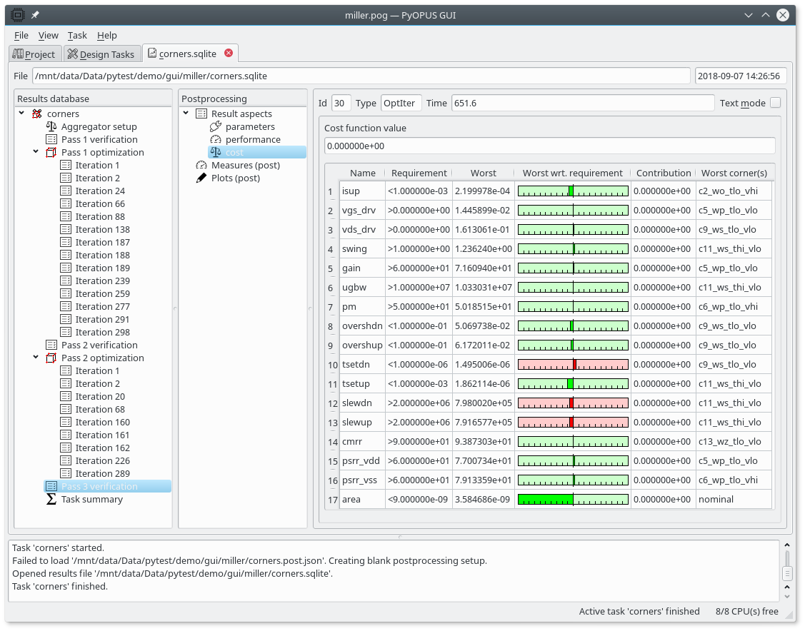
The cost function of the final circuit. Some performance measures do not satisfy the design requirements (tsetdn, slewdn, slewup). Note that they were not subject to optimization (see the Requirements item in the task’s setup).

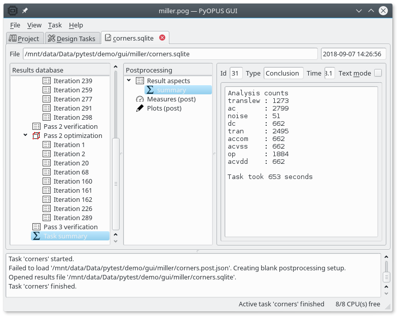
The summary of the optimization run.

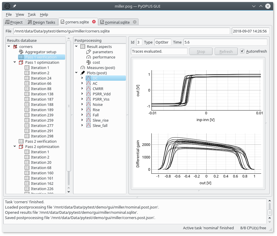
To plot the waveforms open the results of the “nominal” task and copy/paste the postprocessing setup to the Results tab of the “corners” task. Now we can examine the DC response of the initial and the final circuit.

The DC response of the initial circuit.

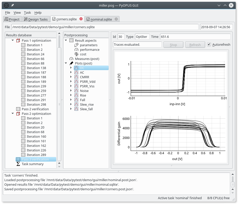
The DC response of the final circuit.

We can see that the spread of the characteristics is much smaller for the final circuit. This is due to the fact that the circuit must satisfy the design requirements across multiple corners. We can also see that the differential gain (>3000) has significantly improved in comparison to the initial circuit (>1500).

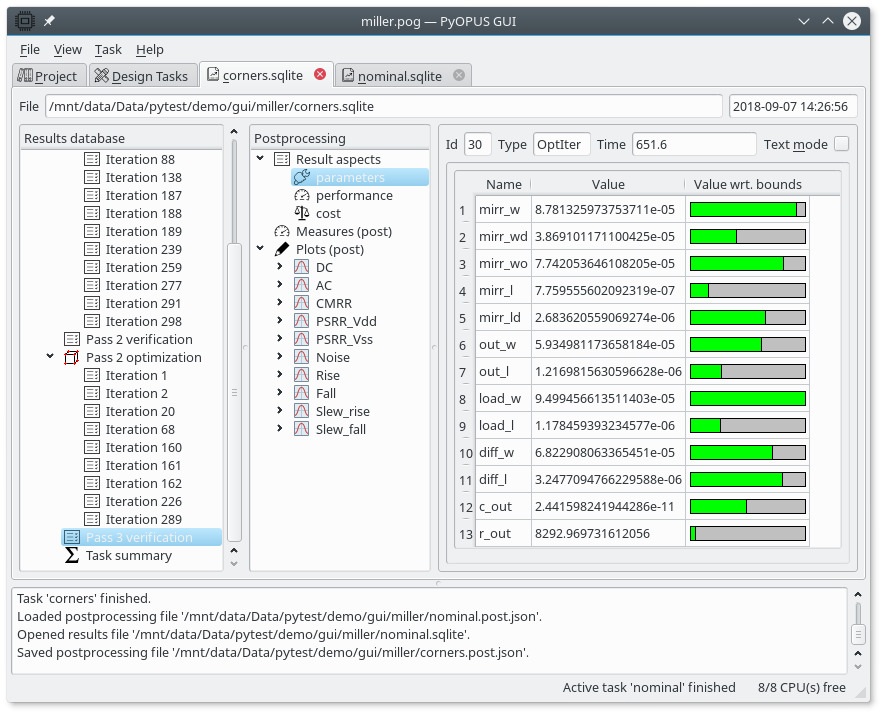
The values of the design parameters for the final circuit.